[TS] HW05

1

\(\{ ε_t \} ∼ W N(0, σ^2_ε)\)이고, \(\{Z_t\}\)에 대하여 다음의 모형을 고려한다.

\[(1 − ϕ_1B − ϕ_2B^2)Z_t = ε_t\]

이 때, \(Z_{n+l}\)의 l−시차 후 MMSE 예측함수 \(Z_n{(l)}\)을 구하여라. 단, 예측함수는 관측값 \(Z_1, . . . , Z_n\)의 함수 형태로 구할 수 있다.

• 위 식은 \(AR(2)\)모형이다.

• (hat생략..)

• \(Z_n(1) = E(Z_{n+1}|Z_n,Z_{n-1},\dots,Z_1) = E(\phi_1 Z_n + \phi_2 Z_{n-1} + \epsilon_{n+1}|Z_n,Z_{n-1},\dots,Z_1)= \phi_1 Z_n + \phi_2 Z_{n-1}\)

• \(Z_n(2) = E(Z_{n+2}|Z_n,Z_{n-1},\dots,Z_1)= E(\phi_1 Z_{n+1} + \phi_2 Z_{n} + \epsilon_{n+2}|Z_n,Z_{n-1},\dots,Z_1) = E(\phi_1 Z_{n+1}|Z_n,Z_{n-1},\dots,Z_1) + \phi_2 Z_n= \phi_1 Z_n(1) + \phi_2 Z_n\)

• \(Z_n(3) = E(Z_{n+3}|Z_n,Z_{n-1},\dots,Z_1)= E(\phi_1 Z_{n+2} + \phi_2 Z_{n+1} + \epsilon_{n+3}|Z_n,Z_{n-1},\dots,Z_1) = \phi_1 Z_n(2) + \phi_2 Z_n(1)\)

• 이를 일반화하면, \(Z_n(l) = \phi_1 Z_n(l-1) + \phi_2 Z_n (l-2)\)이다.

2

어느 시계열자료 \({Z_1, . . . , Z_{100}}\)는 AR(2)모형에 적합되어 모수들의 추정값

\[\hat ϕ_1 = 1.38, \hat ϕ_2 = −0.7, \hat µ = 51.56, \hat σ^2_ε = 4.41\]

을 얻었다. 이 시계열의 마지막 5개 자료는

\[Z_{96} = 52.65, Z_{97} = 54.87, Z_{98} = 53.37, Z_{99} = 48.21, Z_{100} = 44.38\]

이다. 1번의 결과를 이용하여 다음 물음에 답하여라.

(1)

\(Z_{101}, Z_{102}, Z_{103}, Z_{104}, Z_{105}\) 를 예측하여라

문제의 AR(2)은 평균이 있는 모형이다.

즉, 1번의 문제와 비슷하지만 \((1 − ϕ_1B − ϕ_2B^2)(Z_t-\mu)= ε_t\) 이므로

\(Z_n(l) = \phi_1 (Z_n(l-1) +\mu) + \phi_2 (Z_n (l-2) + \mu)\)이므로..

\(Z_{101} = Z_{100}(1) = 1.38 \times (44.38+51.56) - 0.7 \times (48.21 + 51.56)\)

1.38*(44.38+51.56)-0.7*(48.21+51.56)

62.5582

\(Z_{102} = Z_{100}(2) = \hat ϕ_1 (Z_{101}+\hat\mu) + \hat ϕ_2 (Z_{100} +\hat\mu)\)

1.38*(62.5582+51.56) - 0.7*(44.38 + 51.56)

90.325116

\(Z_{103} = Z_{100}(3) = \hat ϕ_1 (Z_{102}+\hat\mu) + \hat ϕ_2( Z_{101} +\hat\mu)\)

1.38*(90.325116+51.56) -0.7* (62.5582 + 51.56)

115.91872008

\(Z_{104} = Z_{100}(4) = \hat ϕ_1 (Z_{103}+\hat\mu) +\hat ϕ_2 (Z_{102} + \hat \mu )\)

1.38*(115.91872008+51.56)-0.7*(90.325116 + 51.56)

131.8010525104

\(Z_{105} = Z_{100}(5) = \hat ϕ_1 (Z_{104}+\hat\mu) +\hat ϕ_2 (Z_{103} + \hat \mu)\)

1.38*(131.8010525104+51.56)-0.7*(115.91872008+51.56)

135.803148408352

(2)

최근에 시점 \(t = 101\)에서 \(Z_{101} = 47.08\)을 얻었다. \(Z_{102}, Z_{103}, Z_{104}, Z_{105}\) 의 예측값을 각각 갱신하여라.

\(Z_{102} = Z_{100}(2) = \hat ϕ_1( Z_{101} + \hat \mu) + \hat ϕ_2( Z_{100} + \hat \mu)\)

1.38*(47.08+51.56)-0.7*(44.38+51.56)

68.9652

\(Z_{103} = Z_{100}(3) = \hat ϕ_1 (Z_{102} + \hat \mu)+ \hat ϕ_2 (Z_{101} + \hat \mu)\)

1.38*(68.9652+51.56)-0.7*(47.08+51.56)

97.276776

\(Z_{104} = Z_{100}(4) = \hat ϕ_1 (Z_{103} + \hat \mu) + \hat ϕ_2 (Z_{102} + \hat \mu)\)

1.38*(97.276776+51.56)-0.7*(68.9652+51.56)

121.02711088

\(Z_{105} = Z_{100}(5) = \hat ϕ_1 (Z_{104} + \hat \mu) + \hat ϕ_2 (Z_{103} + \hat \mu)\)

1.38*(121.02711088+51.56)-0.7*(97.276776+51.56)

133.9844698144

3

(R실습). HW04의 6번에서 적합한 모형에 대하여 마지막 시점 이후 25시점의 값을 예측하고, 예측값과 예측구간을 원시계열 자료의 시계열 그림 위에 겹쳐 그려라.

z6 <- scan("ex8_2b.txt")
forecast::tsdisplay(z6)

Registered S3 method overwritten by 'quantmod':
  method            from
  as.zoo.data.frame zoo 

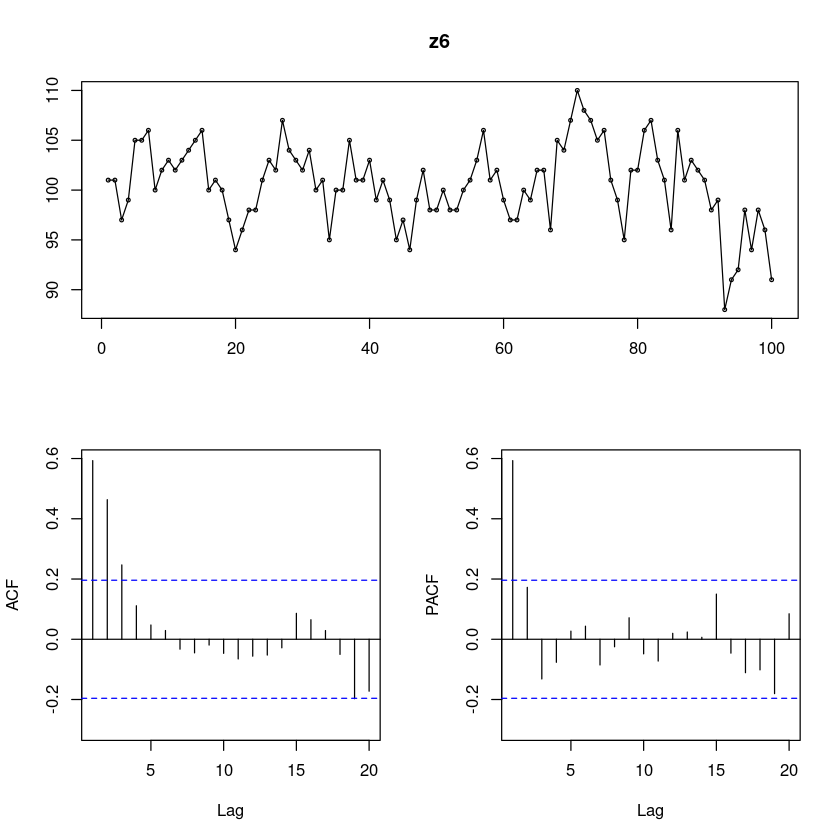
## 모형적합 AR(1)
fit <- arima(z6,order=c(1,0,0))
summary(fit)

Call:
arima(x = z6, order = c(1, 0, 0))

Coefficients:
         ar1  intercept
      0.6231   100.4528
s.e.  0.0805     0.8253

sigma^2 estimated as 9.962:  log likelihood = -257.08,  aic = 520.16

Training set error measures:
                       ME     RMSE      MAE        MPE     MAPE      MASE
Training set -0.004602625 3.156255 2.452284 -0.1060461 2.457104 0.8991709
                  ACF1
Training set -0.100928

forecast_fit <- forecast::forecast(fit, 25) 
forecast_fit

    Point Forecast    Lo 80    Hi 80    Lo 95    Hi 95
101       94.56289 90.51799  98.6078 88.37675 100.7490
102       96.78288 92.01704 101.5487 89.49415 104.0716
103       98.16612 93.14822 103.1840 90.49190 105.8403
104       99.02800 93.91559 104.1404 91.20924 106.8468
105       99.56502 94.41638 104.7137 91.69086 107.4392
106       99.89963 94.73700 105.0623 92.00407 107.7952
107      100.10812 94.94007 105.2762 92.20427 108.0120
108      100.23803 95.06787 105.4082 92.33096 108.1451
109      100.31897 95.14800 105.4899 92.41065 108.2273
110      100.36941 95.19812 105.5407 92.46060 108.2782
111      100.40083 95.22942 105.5722 92.49184 108.3098
112      100.42041 95.24895 105.5919 92.51134 108.3295
113      100.43261 95.26113 105.6041 92.52352 108.3417
114      100.44022 95.26873 105.6117 92.53111 108.3493
115      100.44495 95.27346 105.6164 92.53584 108.3541
116      100.44790 95.27641 105.6194 92.53879 108.3570
117      100.44974 95.27825 105.6212 92.54063 108.3589
118      100.45089 95.27940 105.6224 92.54177 108.3600
119      100.45160 95.28011 105.6231 92.54249 108.3607
120      100.45205 95.28055 105.6235 92.54293 108.3612
121      100.45232 95.28083 105.6238 92.54321 108.3614
122      100.45250 95.28100 105.6240 92.54338 108.3616
123      100.45260 95.28111 105.6241 92.54349 108.3617
124      100.45267 95.28118 105.6242 92.54356 108.3618
125      100.45271 95.28122 105.6242 92.54360 108.3618

plot(forecast_fit)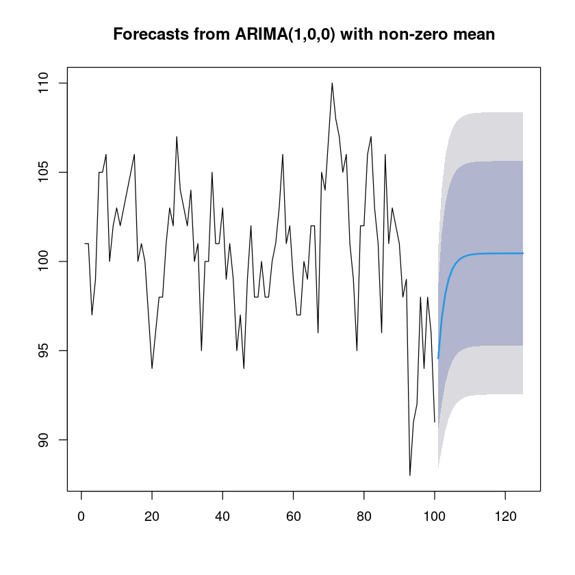

## 모형적합 ARMA(1,2)
fitt <- arima(z6,order=c(1,0,2))
summary(fitt)
forecast_fitt <- forecast::forecast(fitt, 25) 
forecast_fitt
plot(forecast_fitt)

Call:
arima(x = z6, order = c(1, 0, 2))

Coefficients:
         ar1      ma1     ma2  intercept
      0.5368  -0.0066  0.2947   100.4720
s.e.  0.1644   0.1651  0.1335     0.8385

sigma^2 estimated as 9.348:  log likelihood = -253.99,  aic = 517.99

Training set error measures:
                      ME     RMSE      MAE        MPE     MAPE      MASE
Training set -0.01379953 3.057498 2.356181 -0.1089919 2.361273 0.8639331
                    ACF1
Training set 0.007421317

    Point Forecast    Lo 80     Hi 80    Lo 95    Hi 95
101       94.94724 91.02890  98.86559 88.95466 100.9398
102       95.40892 90.97386  99.84397 88.62609 102.1917
103       97.75397 92.77164 102.73630 90.13416 105.3738
104       99.01288 93.88365 104.14210 91.16841 106.8573
105       99.68870 94.51792 104.85948 91.78067 107.5967
106      100.05150 94.86881 105.23420 92.12526 107.9777
107      100.24627 95.06015 105.43239 92.31478 108.1778
108      100.35083 95.16372 105.53794 92.41783 108.2838
109      100.40696 95.21956 105.59435 92.47352 108.3404
110      100.43709 95.24961 105.62456 92.50353 108.3706
111      100.45326 95.26576 105.64076 92.51967 108.3869
112      100.46195 95.27444 105.64945 92.52834 108.3956
113      100.46661 95.27910 105.65412 92.53300 108.4002
114      100.46911 95.28160 105.65662 92.53550 108.4027
115      100.47046 95.28295 105.65797 92.53684 108.4041
116      100.47118 95.28367 105.65869 92.53757 108.4048
117      100.47156 95.28405 105.65907 92.53795 108.4052
118      100.47177 95.28426 105.65928 92.53816 108.4054
119      100.47188 95.28437 105.65939 92.53827 108.4055
120      100.47194 95.28443 105.65945 92.53833 108.4056
121      100.47198 95.28447 105.65949 92.53836 108.4056
122      100.47199 95.28448 105.65950 92.53838 108.4056
123      100.47200 95.28449 105.65951 92.53839 108.4056
124      100.47201 95.28450 105.65952 92.53840 108.4056
125      100.47201 95.28450 105.65952 92.53840 108.4056

4__다시다시

(R실습). ex10_41.txt, ex10_4b.txt 자료는 어느 확률과정으로부터 생성된 모의 실험자료이다.

• ex10_4a인듯?

(1)

각 시계열 \(\{Z_t \}\)의 시계열 그림을 그려라.

z4a <- scan("ex10_4a.txt")
forecast::tsdisplay(z4a, lag.max=30)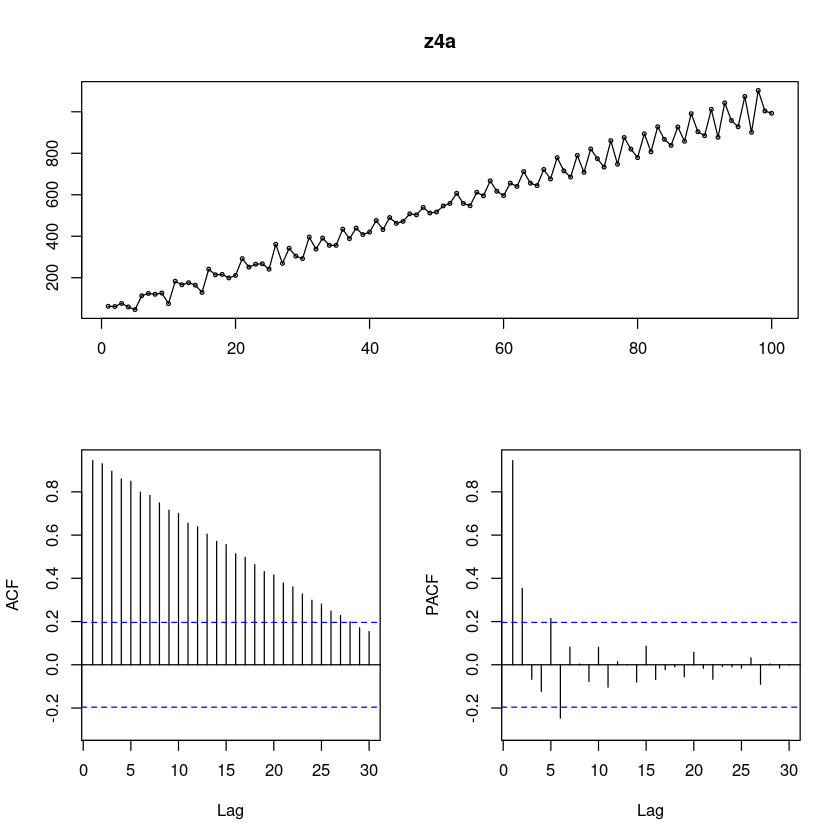

• 시도표를 확인해보니 추세가 있어보인다. 시간이 지날수록 분산이 조금씩 커지는 것 같다. 계절성분은.. 없어보인다.

• ACF는 점점 감소하고 있다.(확률적 추세)

• PACF는 2차시까지 살아있는 것 같고.. (5차시와 6차시가 조금 튀어나왔지만 무시할만하다..)

• AR(2)모형인가?

z4b <- scan("ex10_4b.txt")
forecast::tsdisplay(z4b)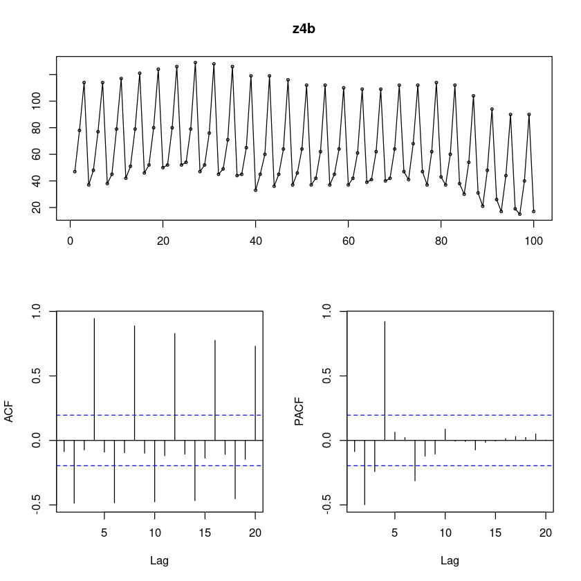

• 계절성분이 있어보인다. 시도표 자체가 흐물흐물

• ACF sin함수? 그리면서 지수적으로 감소하는 듯 하다. 길게보니까 천천히 감소하는 것 같기도…

• PACF는.. 2차시…4차시.. 6차시가 살아있고

• PACF가 4이후에 절단된 형태이다.

• ARIMA(0,0,0)(1,0,0)_4 로 보이기도 하네

(2)

각 시계열 \(\{Z_t\}\)의 SACF와 SPACF를 그려라

(1)과 동일. 생략

(3)

각 시계열이 정상시계열이 되도록 적절한 변환 혹은 차분을 단계적으로 취하여라

z4a

log_z4a = log(z4a)
sqrt_z4a = sqrt(z4a)
boxcox_z4a = forecast::BoxCox(z4a,lambda= forecast::BoxCox.lambda(z4a))

par(mfrow=c(2,2))
plot.ts(z4a, main = "original")
plot.ts(log_z4a, main = 'log')
plot.ts(sqrt_z4a, main = 'sqrt')
plot.ts(boxcox_z4a, main = 'Boxcox')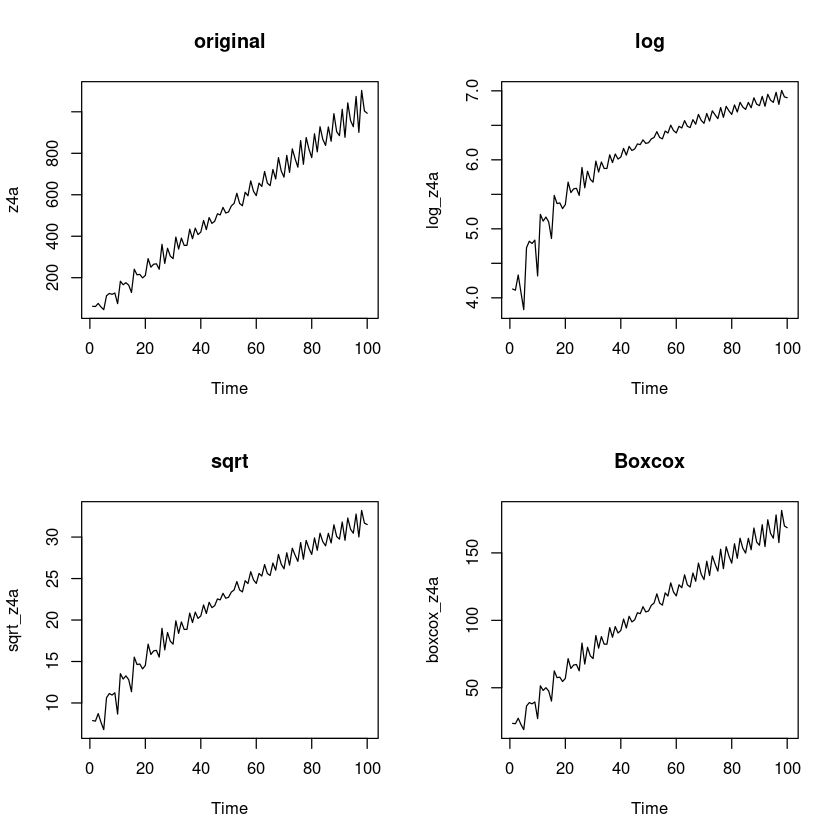

t4a = 1:length(z4a)
lmtest::bptest(lm(z4a~t4a)) #H0 : 등분산이다
lmtest::bptest(lm(log_z4a~t4a))
lmtest::bptest(lm(sqrt_z4a~t4a))
lmtest::bptest(lm(boxcox_z4a~t4a))

    studentized Breusch-Pagan test

data:  lm(z4a ~ t4a)
BP = 24.415, df = 1, p-value = 7.765e-07

    studentized Breusch-Pagan test

data:  lm(log_z4a ~ t4a)
BP = 13.279, df = 1, p-value = 0.0002684

    studentized Breusch-Pagan test

data:  lm(sqrt_z4a ~ t4a)
BP = 5.5272, df = 1, p-value = 0.01872

    studentized Breusch-Pagan test

data:  lm(boxcox_z4a ~ t4a)
BP = 0.065359, df = 1, p-value = 0.7982

• boxcox하는 것이 등분산이니까.. boxcox한걸로 하자.

##단위근 검정 : H0 : 단위근이 있다.
fUnitRoots::adfTest(z4a, lags = 0, type = "c")
fUnitRoots::adfTest(z4a, lags = 6, type = "c")
fUnitRoots::adfTest(z4a, lags = 12, type = "c")

Title:
 Augmented Dickey-Fuller Test

Test Results:
  PARAMETER:
    Lag Order: 0
  STATISTIC:
    Dickey-Fuller: -1.2765
  P VALUE:
    0.5828 

Description:
 Tue Dec 12 16:40:17 2023 by user: 

Title:
 Augmented Dickey-Fuller Test

Test Results:
  PARAMETER:
    Lag Order: 6
  STATISTIC:
    Dickey-Fuller: -0.5851
  P VALUE:
    0.8387 

Description:
 Tue Dec 12 16:40:17 2023 by user: 

Title:
 Augmented Dickey-Fuller Test

Test Results:
  PARAMETER:
    Lag Order: 12
  STATISTIC:
    Dickey-Fuller: -1.1272
  P VALUE:
    0.638 

Description:
 Tue Dec 12 16:40:17 2023 by user: 

• P-value의 값이 0.05보다 크므로 h0를 기각할 수 없다. 즉 차분이 필요하다.

forecast::tsdisplay(boxcox_z4a)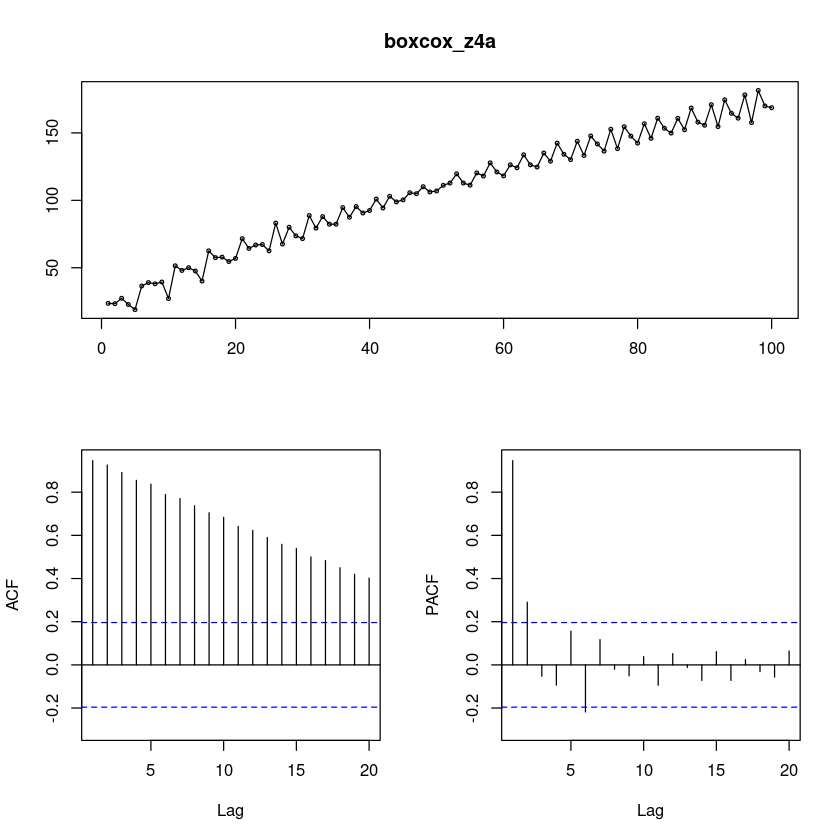

• ACF에서 천천히 감소하는 확률적 추세를 보이니까 차분을 해보아야겠다! 계절은 솔직히 좀 애매해보인다.

diff_boxcox_z4a = diff(boxcox_z4a)
forecast::tsdisplay(diff_boxcox_z4a,lag.max=100)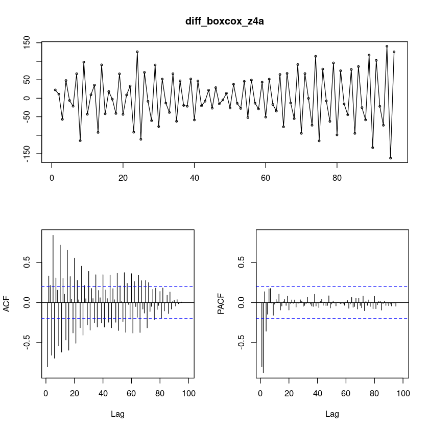

• 차분을 했더니 계절성분이 더 잘 보인다. 지수적으로 감소하지만 중간에 튀어나온 부분이 있다.

• 단위근 검정을 통해서 왜 차분할 필요가 없다고 뜨지? (궁금…)

- 주기가 5로 보여서 5로 했음.

lag5_diff_boxcox_z4a = diff(diff(boxcox_z4a),5)
forecast::tsdisplay(lag5_diff_boxcox_z4a, lag.max=60)

• 상수항이 없는 AIRMA(0,0,3)(0,0,1)_5 같이 보인다..

z4b

log_z4b = log(z4b)
sqrt_z4b = sqrt(z4b)
boxcox_z4b = forecast::BoxCox(z4b,lambda= forecast::BoxCox.lambda(z4b))

par(mfrow=c(2,2))
plot.ts(z4b, main = "original")
plot.ts(log_z4b, main = 'log')
plot.ts(sqrt_z4b, main = 'sqrt')
plot.ts(boxcox_z4b, main = 'Boxcox')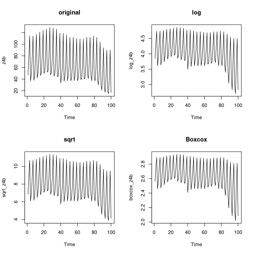

t4b = 1:length(z4b)
lmtest::bptest(lm(z4b~t4b)) #H0 : 등분산이다
lmtest::bptest(lm(log_z4b~t4b))
lmtest::bptest(lm(sqrt_z4b~t4b))
lmtest::bptest(lm(boxcox_z4b~t4b))

    studentized Breusch-Pagan test

data:  lm(z4b ~ t4b)
BP = 0.0077657, df = 1, p-value = 0.9298

    studentized Breusch-Pagan test

data:  lm(log_z4b ~ t4b)
BP = 8.6591, df = 1, p-value = 0.003254

    studentized Breusch-Pagan test

data:  lm(sqrt_z4b ~ t4b)
BP = 1.6816, df = 1, p-value = 0.1947

    studentized Breusch-Pagan test

data:  lm(boxcox_z4b ~ t4b)
BP = 12.23, df = 1, p-value = 0.0004702

• 원데이터가 제일 P-value가 높다. 원데이터를 사용해도 좋고.. y값의 범위가 크므로 sqrt변환한 것을 사용해도 좋을 것 같다.

lag4_sqrt_z4b = diff(sqrt_z4b, 4)
forecast::tsdisplay(lag4_sqrt_z4b)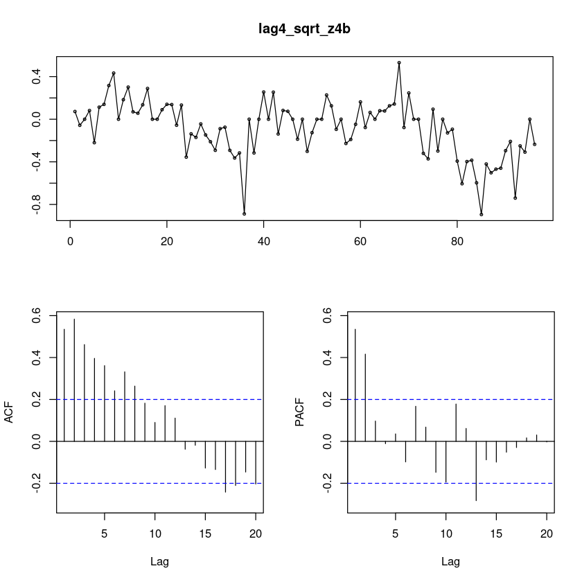

##단위근 검정 : H0 : 단위근이 있다.
fUnitRoots::adfTest(lag4_sqrt_z4b, lags = 1, type = "c")
fUnitRoots::adfTest(lag4_sqrt_z4b, lags = 2, type = "c")
fUnitRoots::adfTest(lag4_sqrt_z4b, lags = 3, type = "c")

Title:
 Augmented Dickey-Fuller Test

Test Results:
  PARAMETER:
    Lag Order: 1
  STATISTIC:
    Dickey-Fuller: -2.9496
  P VALUE:
    0.04505 

Description:
 Wed Dec 13 09:49:20 2023 by user: 

Title:
 Augmented Dickey-Fuller Test

Test Results:
  PARAMETER:
    Lag Order: 2
  STATISTIC:
    Dickey-Fuller: -2.5309
  P VALUE:
    0.1189 

Description:
 Wed Dec 13 09:49:20 2023 by user: 

Title:
 Augmented Dickey-Fuller Test

Test Results:
  PARAMETER:
    Lag Order: 3
  STATISTIC:
    Dickey-Fuller: -2.4565
  P VALUE:
    0.1464 

Description:
 Wed Dec 13 09:49:20 2023 by user: 

• p-value값 애매하지만. 단위근이 있다고 판단하고 차분을 한 번 더 해보자

diff_lag4_sqrt_z4b = diff(diff(lag4_sqrt_z4b, 4))
forecast::tsdisplay(diff_lag4_sqrt_z4b,lag.max=70)

(4)

적절한 모형을 식별하여 적합하여라

z4a

lag5_diff_boxcox_z4a = diff(diff(boxcox_z4a),5)
forecast::tsdisplay(lag5_diff_boxcox_z4a, lag.max=60)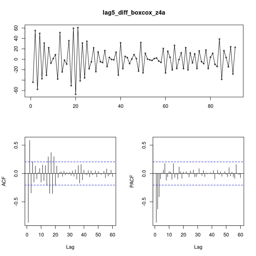

• 상수항이 없는 AIRMA(3,0,0)(0,1,1)_5 같이 보인다..

lag5_diff_boxcox_z = \(ARIMA(3,0,0)(0,1,1)_{5}\)

t.test(lag5_diff_boxcox_z4a)

    One Sample t-test

data:  lag5_diff_boxcox_z4a
t = -0.038719, df = 90, p-value = 0.9692
alternative hypothesis: true mean is not equal to 0
95 percent confidence interval:
 -5.443111  5.235003
sample estimates:
 mean of x 
-0.1040539 

- 모형1(내가 생각한)

fit11 = arima(lag5_diff_boxcox_z4a, order = c(3,0,0), include.mean=F,
     seasonal = list(order = c(0,1,1), period=5))
summary(fit11)
lmtest::coeftest(fit11) 

Call:
arima(x = lag5_diff_boxcox_z4a, order = c(3, 0, 0), seasonal = list(order = c(0, 
    1, 1), period = 5), include.mean = F)

Coefficients:
          ar1      ar2      ar3    sma1
      -1.8850  -1.5761  -0.6237  -1.000
s.e.   0.0823   0.1347   0.0830   0.145

sigma^2 estimated as 48.66:  log likelihood = -299,  aic = 608

Training set error measures:
                   ME     RMSE      MAE      MPE     MAPE      MASE       ACF1
Training set 0.212755 6.781579 5.107949 40.42187 92.98714 0.1347569 -0.2943703

z test of coefficients:

      Estimate Std. Error  z value  Pr(>|z|)    
ar1  -1.885039   0.082273 -22.9119 < 2.2e-16 ***
ar2  -1.576098   0.134729 -11.6983 < 2.2e-16 ***
ar3  -0.623737   0.083004  -7.5145 5.712e-14 ***
sma1 -0.999999   0.145009  -6.8961 5.344e-12 ***
---
Signif. codes:  0 ‘***’ 0.001 ‘**’ 0.01 ‘*’ 0.05 ‘.’ 0.1 ‘ ’ 1

음.. 근데 또 생각해보니 주기가 5인디.. ma1,ma2,ma3,sma1이 의미가 있남??

- 모형2(AUTO)

fit12 <- forecast::auto.arima(ts(boxcox_z4a, frequency=5),
                     test = "adf",
                     seasonal = TRUE, trace = T)

 ARIMA(2,0,2)(1,1,1)[5] with drift         : Inf
 ARIMA(0,0,0)(0,1,0)[5] with drift         : 740.7953
 ARIMA(1,0,0)(1,1,0)[5] with drift         : 626.1767
 ARIMA(0,0,1)(0,1,1)[5] with drift         : Inf
 ARIMA(0,0,0)(0,1,0)[5]                    : 738.7131
 ARIMA(1,0,0)(0,1,0)[5] with drift         : 624.2993
 ARIMA(1,0,0)(0,1,1)[5] with drift         : 625.7293
 ARIMA(1,0,0)(1,1,1)[5] with drift         : Inf
 ARIMA(2,0,0)(0,1,0)[5] with drift         : 584.0149
 ARIMA(2,0,0)(1,1,0)[5] with drift         : 585.8908
 ARIMA(2,0,0)(0,1,1)[5] with drift         : 585.3023
 ARIMA(2,0,0)(1,1,1)[5] with drift         : 584.8715
 ARIMA(3,0,0)(0,1,0)[5] with drift         : 551.7999
 ARIMA(3,0,0)(1,1,0)[5] with drift         : 549.1616
 ARIMA(3,0,0)(2,1,0)[5] with drift         : 544.3506
 ARIMA(3,0,0)(2,1,1)[5] with drift         : Inf
 ARIMA(3,0,0)(1,1,1)[5] with drift         : Inf
 ARIMA(2,0,0)(2,1,0)[5] with drift         : 578.1867
 ARIMA(4,0,0)(2,1,0)[5] with drift         : 520.1342
 ARIMA(4,0,0)(1,1,0)[5] with drift         : 528.2307
 ARIMA(4,0,0)(2,1,1)[5] with drift         : 513.4132
 ARIMA(4,0,0)(1,1,1)[5] with drift         : Inf
 ARIMA(4,0,0)(2,1,2)[5] with drift         : Inf
 ARIMA(4,0,0)(1,1,2)[5] with drift         : 513.3994
 ARIMA(4,0,0)(0,1,2)[5] with drift         : Inf
 ARIMA(4,0,0)(0,1,1)[5] with drift         : 510.9336
 ARIMA(4,0,0)(0,1,0)[5] with drift         : 532.0723
 ARIMA(3,0,0)(0,1,1)[5] with drift         : Inf
 ARIMA(4,0,1)(0,1,1)[5] with drift         : Inf
 ARIMA(3,0,1)(0,1,1)[5] with drift         : Inf
 ARIMA(4,0,0)(0,1,1)[5]                    : 508.5887
 ARIMA(4,0,0)(0,1,0)[5]                    : 529.7897
 ARIMA(4,0,0)(1,1,1)[5]                    : Inf
 ARIMA(4,0,0)(0,1,2)[5]                    : Inf
 ARIMA(4,0,0)(1,1,0)[5]                    : 525.8971
 ARIMA(4,0,0)(1,1,2)[5]                    : 510.9393
 ARIMA(3,0,0)(0,1,1)[5]                    : Inf
 ARIMA(4,0,1)(0,1,1)[5]                    : Inf
 ARIMA(3,0,1)(0,1,1)[5]                    : Inf

 Best model: ARIMA(4,0,0)(0,1,1)[5]                    

summary(fit12)
lmtest::coeftest(fit12) 

Series: ts(boxcox_z4a, frequency = 5) 
ARIMA(4,0,0)(0,1,1)[5] 

Coefficients:
          ar1      ar2      ar3      ar4    sma1
      -2.1667  -2.3899  -1.6894  -0.5040  0.8504
s.e.   0.0887   0.1687   0.1721   0.0903  0.1266

sigma^2 = 12.41:  log likelihood = -247.8
AIC=507.6   AICc=508.59   BIC=522.73

Training set error measures:
                     ME     RMSE      MAE      MPE     MAPE      MASE
Training set 0.02965456 3.336453 2.523371 240.7739 267.0698 0.2449732
                   ACF1
Training set -0.1173739

z test of coefficients:

      Estimate Std. Error  z value  Pr(>|z|)    
ar1  -2.166679   0.088716 -24.4226 < 2.2e-16 ***
ar2  -2.389871   0.168724 -14.1644 < 2.2e-16 ***
ar3  -1.689432   0.172074  -9.8180 < 2.2e-16 ***
ar4  -0.503953   0.090284  -5.5819 2.380e-08 ***
sma1  0.850377   0.126584   6.7179 1.844e-11 ***
---
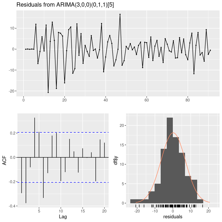
Signif. codes:  0 ‘***’ 0.001 ‘**’ 0.01 ‘*’ 0.05 ‘.’ 0.1 ‘ ’ 1

• auto로 적합한 모형의 AIC도 낮고.. 각 계수들도 유의해서 괜찮은 것 같다. 그런데 모형 자체가 너무 복잡한듯!

잔차분석

forecast::checkresiduals(fit11)

    Ljung-Box test

data:  Residuals from ARIMA(3,0,0)(0,1,1)[5]
Q* = 61.287, df = 6, p-value = 2.464e-11

Model df: 4.   Total lags used: 10

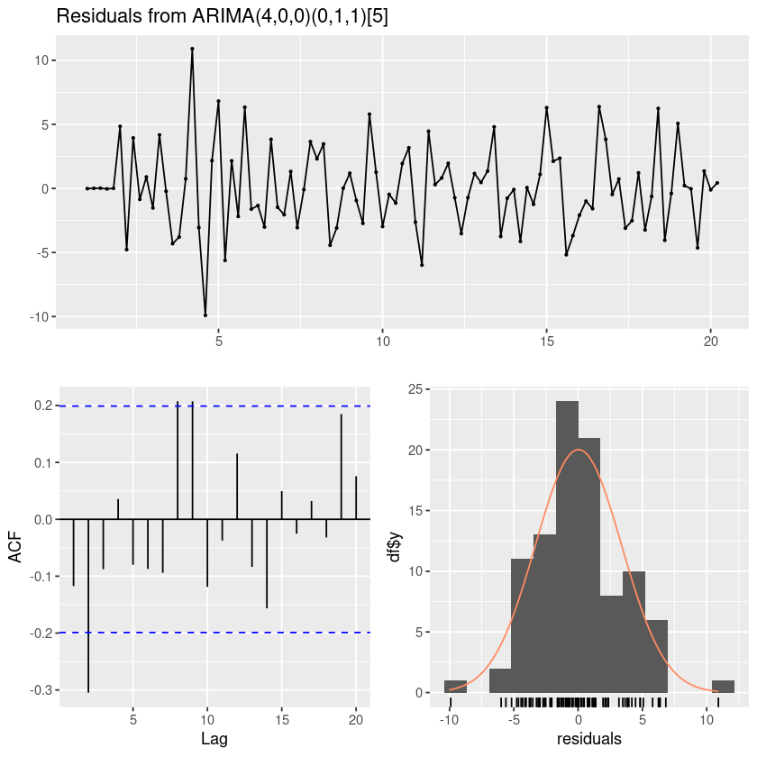
forecast::checkresiduals(fit12)

    Ljung-Box test

data:  Residuals from ARIMA(4,0,0)(0,1,1)[5]
Q* = 24.986, df = 5, p-value = 0.0001402

Model df: 5.   Total lags used: 10

t.test(resid(fit11))

    One Sample t-test

data:  resid(fit11)
t = 0.29777, df = 90, p-value = 0.7666
alternative hypothesis: true mean is not equal to 0
95 percent confidence interval:
 -1.206703  1.632213
sample estimates:
mean of x 
 0.212755 

t.test(resid(fit12))

    One Sample t-test

data:  resid(fit12)
t = 0.087088, df = 96, p-value = 0.9308
alternative hypothesis: true mean is not equal to 0
95 percent confidence interval:
 -0.6462561  0.7055652
sample estimates:
 mean of x 
0.02965456 

• 잔차의 평균은 0이다.

#모형 적합도 검정 : H0 : rho1=...=rho_k=0
Box.test(resid(fit11), lag=1, type = "Ljung-Box")
Box.test(resid(fit11), lag=2, type = "Ljung-Box")
Box.test(resid(fit11), lag=5, type = "Ljung-Box")

    Box-Ljung test

data:  resid(fit11)
X-squared = 8.1484, df = 1, p-value = 0.00431

    Box-Ljung test

data:  resid(fit11)
X-squared = 21.629, df = 2, p-value = 2.01e-05

    Box-Ljung test

data:  resid(fit11)
X-squared = 36.991, df = 5, p-value = 6.015e-07

• WN이 아니당..

#모형 적합도 검정 : H0 : rho1=...=rho_k=0
Box.test(resid(fit12), lag=1, type = "Ljung-Box")
Box.test(resid(fit12), lag=6, type = "Ljung-Box")
Box.test(resid(fit12), lag=12, type = "Ljung-Box")

    Box-Ljung test

data:  resid(fit12)
X-squared = 1.3781, df = 1, p-value = 0.2404

    Box-Ljung test

data:  resid(fit12)
X-squared = 13.15, df = 6, p-value = 0.04071

    Box-Ljung test

data:  resid(fit12)
X-squared = 26.651, df = 12, p-value = 0.008672

• WN이다. fit12를 선택하는 것이 적절해 보인다.

z4b

forecast::tsdisplay(diff_lag4_sqrt_z4b,lag.max=70)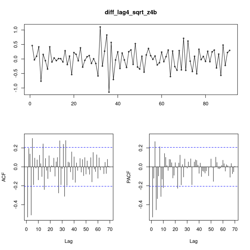

• SMA(1)?

• ARIMA(0,1,1)(0,1,1)_5

- 모형1(내가 생각한)

fit11 = arima(diff_lag4_sqrt_z4b, order = c(0,1,1), include.mean=F,
     seasonal = list(order = c(0,1,1), period=4))
summary(fit11)
lmtest::coeftest(fit11) 

Call:
arima(x = diff_lag4_sqrt_z4b, order = c(0, 1, 1), seasonal = list(order = c(0, 
    1, 1), period = 4), include.mean = F)

Coefficients:
          ma1     sma1
      -1.0000  -1.0000
s.e.   0.0469   0.0655

sigma^2 estimated as 0.1375:  log likelihood = -47.09,  aic = 100.19

Training set error measures:
                     ME      RMSE       MAE      MPE     MAPE      MASE
Training set 0.04078458 0.3604663 0.2723856 112.9697 122.2518 0.5489001
                   ACF1
Training set -0.4989492

z test of coefficients:

      Estimate Std. Error z value  Pr(>|z|)    
ma1  -1.000000   0.046855 -21.343 < 2.2e-16 ***
sma1 -0.999999   0.065499 -15.267 < 2.2e-16 ***
---
Signif. codes:  0 ‘***’ 0.001 ‘**’ 0.01 ‘*’ 0.05 ‘.’ 0.1 ‘ ’ 1

- 모형2(AUTO)

fit123 <- forecast::auto.arima(ts(sqrt_z4b, frequency=4),
                     test = "adf",
                     seasonal = TRUE, trace = T)
summary(fit123)
lmtest::coeftest(fit123)

 ARIMA(2,0,2)(1,1,1)[4] with drift         : -20.17843
 ARIMA(0,0,0)(0,1,0)[4] with drift         : 17.47937
 ARIMA(1,0,0)(1,1,0)[4] with drift         : -11.73833
 ARIMA(0,0,1)(0,1,1)[4] with drift         : -1.067821
 ARIMA(0,0,0)(0,1,0)[4]                    : 26.30471
 ARIMA(2,0,2)(0,1,1)[4] with drift         : -22.41085
 ARIMA(2,0,2)(0,1,0)[4] with drift         : -24.73603
 ARIMA(2,0,2)(1,1,0)[4] with drift         : -22.41257
 ARIMA(1,0,2)(0,1,0)[4] with drift         : -26.75223
 ARIMA(1,0,2)(1,1,0)[4] with drift         : -24.48929
 ARIMA(1,0,2)(0,1,1)[4] with drift         : -24.48391
 ARIMA(1,0,2)(1,1,1)[4] with drift         : -24.93594
 ARIMA(0,0,2)(0,1,0)[4] with drift         : -12.89084
 ARIMA(1,0,1)(0,1,0)[4] with drift         : -26.06203
 ARIMA(1,0,3)(0,1,0)[4] with drift         : -24.76333
 ARIMA(0,0,1)(0,1,0)[4] with drift         : 2.74682
 ARIMA(0,0,3)(0,1,0)[4] with drift         : -20.00937
 ARIMA(2,0,1)(0,1,0)[4] with drift         : -26.99294
 ARIMA(2,0,1)(1,1,0)[4] with drift         : -24.73092
 ARIMA(2,0,1)(0,1,1)[4] with drift         : -24.72671
 ARIMA(2,0,1)(1,1,1)[4] with drift         : -22.56032
 ARIMA(2,0,0)(0,1,0)[4] with drift         : -28.39065
 ARIMA(2,0,0)(1,1,0)[4] with drift         : -26.19614
 ARIMA(2,0,0)(0,1,1)[4] with drift         : -26.18687
 ARIMA(2,0,0)(1,1,1)[4] with drift         : -23.96165
 ARIMA(1,0,0)(0,1,0)[4] with drift         : -12.66527
 ARIMA(3,0,0)(0,1,0)[4] with drift         : -27.03259
 ARIMA(3,0,1)(0,1,0)[4] with drift         : -25.61228
 ARIMA(2,0,0)(0,1,0)[4]                    : -29.19281
 ARIMA(2,0,0)(1,1,0)[4]                    : -27.0484
 ARIMA(2,0,0)(0,1,1)[4]                    : -27.03837
 ARIMA(2,0,0)(1,1,1)[4]                    : -24.86536
 ARIMA(1,0,0)(0,1,0)[4]                    : -11.61871
 ARIMA(3,0,0)(0,1,0)[4]                    : -28.0884
 ARIMA(2,0,1)(0,1,0)[4]                    : -28.08562
 ARIMA(1,0,1)(0,1,0)[4]                    : -27.25033
 ARIMA(3,0,1)(0,1,0)[4]                    : -25.8663

 Best model: ARIMA(2,0,0)(0,1,0)[4]                    

Series: ts(sqrt_z4b, frequency = 4) 
ARIMA(2,0,0)(0,1,0)[4] 

Coefficients:
         ar1     ar2
      0.3275  0.4291
s.e.  0.0913  0.0912

sigma^2 = 0.04099:  log likelihood = 17.73
AIC=-29.45   AICc=-29.19   BIC=-21.76

Training set error measures:
                     ME      RMSE       MAE        MPE     MAPE      MASE
Training set -0.0227614 0.1962891 0.1472304 -0.4922113 2.155832 0.7396851
                    ACF1
Training set -0.05524958

z test of coefficients:

    Estimate Std. Error z value  Pr(>|z|)    
ar1 0.327459   0.091311  3.5862 0.0003355 ***
ar2 0.429138   0.091227  4.7041  2.55e-06 ***
---
Signif. codes:  0 ‘***’ 0.001 ‘**’ 0.01 ‘*’ 0.05 ‘.’ 0.1 ‘ ’ 1

잔차분석

forecast::checkresiduals(fit11)

    Ljung-Box test

data:  Residuals from ARIMA(3,0,0)(0,1,1)[5]
Q* = 61.287, df = 6, p-value = 2.464e-11

Model df: 4.   Total lags used: 10

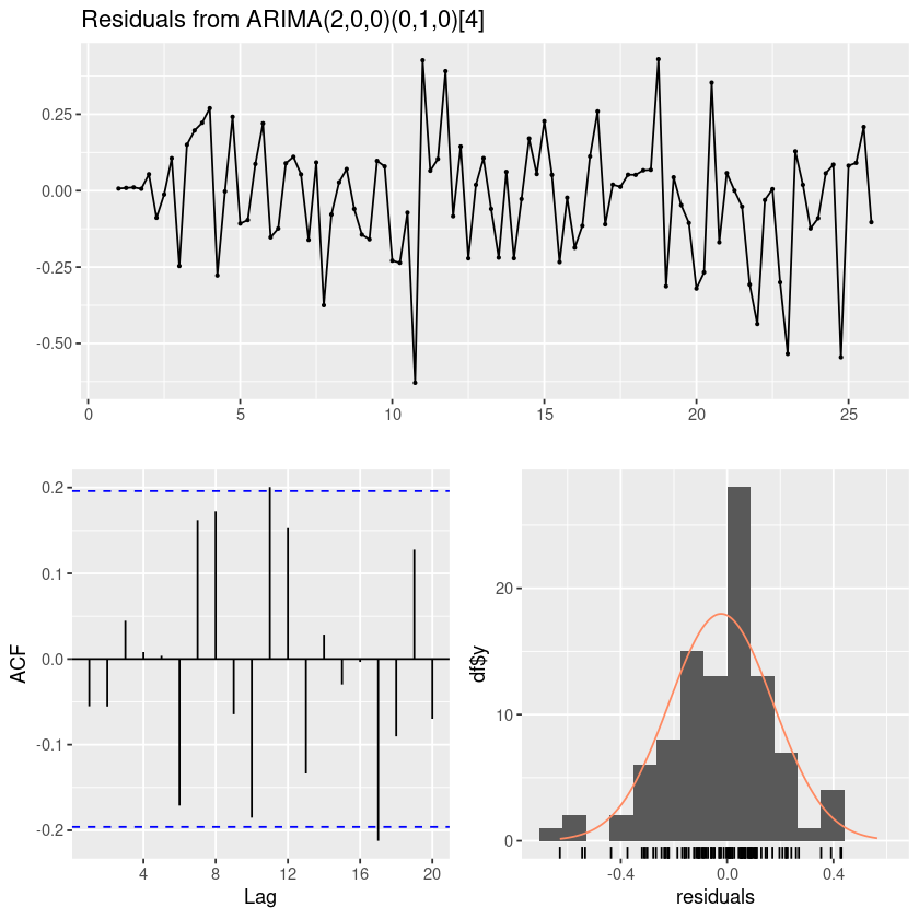
forecast::checkresiduals(fit123)

    Ljung-Box test

data:  Residuals from ARIMA(2,0,0)(0,1,0)[4]
Q* = 10.212, df = 6, p-value = 0.116

Model df: 2.   Total lags used: 8

#모형 적합도 검정 : H0 : rho1=...=rho_k=0
Box.test(resid(fit11), lag=1, type = "Ljung-Box")
Box.test(resid(fit11), lag=2, type = "Ljung-Box")
Box.test(resid(fit11), lag=5, type = "Ljung-Box")

    Box-Ljung test

data:  resid(fit11)
X-squared = 8.1484, df = 1, p-value = 0.00431

    Box-Ljung test

data:  resid(fit11)
X-squared = 21.629, df = 2, p-value = 2.01e-05

    Box-Ljung test

data:  resid(fit11)
X-squared = 36.991, df = 5, p-value = 6.015e-07

#모형 적합도 검정 : H0 : rho1=...=rho_k=0
Box.test(resid(fit123), lag=1, type = "Ljung-Box")
Box.test(resid(fit123), lag=2, type = "Ljung-Box")
Box.test(resid(fit123), lag=5, type = "Ljung-Box")

    Box-Ljung test

data:  resid(fit123)
X-squared = 0.3145, df = 1, p-value = 0.5749

    Box-Ljung test

data:  resid(fit123)
X-squared = 0.63453, df = 2, p-value = 0.7281

    Box-Ljung test

data:  resid(fit123)
X-squared = 0.85341, df = 5, p-value = 0.9735

• ㅜㅜ auto가 더 낫다.. 계절형 ARIMA모델은 너무 어려워

(5)

위에서 적합한 결과를 이용하여, n = 10000으로 하여 새로운 모의실험 자료를 생성하여 (2)번에서의 SACF와 SPACF를 비교하여라

### ARIMA(p,d,q)(P,D,Q)_s  (z4a)

ars <- c(-2.166679, -2.389871, -1.689432, -0.503953)
sma <- 0.850377
x <- sarima::sim_sarima(n=10000,  model=list(ar = ars, sma=sma), nseasons=5) 
forecast::tsdisplay(x)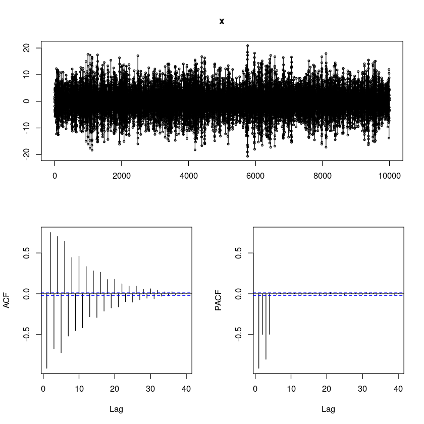

### ARIMA(p,d,q)(P,D,Q)_s  (z4b)

ars <- c(0.3275, 0.4291)
x <- sarima::sim_sarima(n=10000,  model=list(ar = ars), nseasons=4) 
forecast::tsdisplay(x)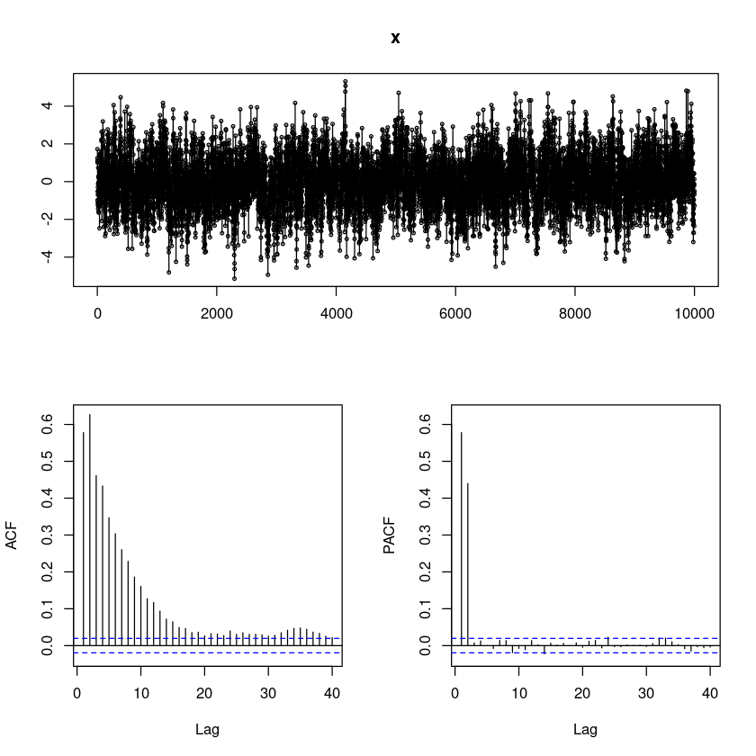

5

(R실습). 1973년 이후 미국에서 단독 주택의 월별 거래량 데이터(fma::hsales)에 대하여 다음 물음에 답하여라.

install.packages("fma")

Installing package into ‘/home/coco/R/x86_64-pc-linux-gnu-library/4.2’
(as ‘lib’ is unspecified)

library(fma)

Loading required package: forecast

str(hsales)

 Time-Series [1:275] from 1973 to 1996: 55 60 68 63 65 61 54 52 46 42 ...

(1)

시계열 그림을 그리시오

forecast::tsdisplay(hsales)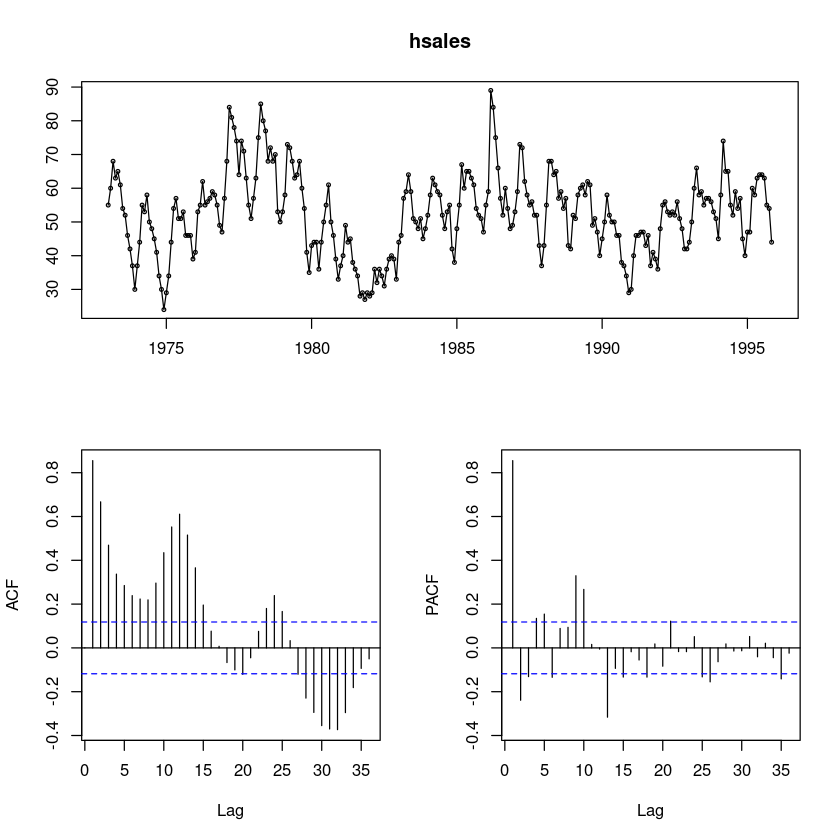

• ACF가 감소하다가 중간에 튀어나오는 부분이 있어 계절성분이 있어 보인다.

• PACF는 1차 이후 중간중간 유의한 부분이 보인다. 계절차분이 필요하다.

(2)

변수변환이 필요한지를 설명하고, 필요하다면 적절한 변수 변환을 하여라.

log_hsales = log(hsales)
sqrt_hsales = sqrt(hsales)
boxcox_hsales = forecast::BoxCox(hsales,lambda= forecast::BoxCox.lambda(hsales))

forecast::BoxCox.lambda(hsales)

0.1454607801013

par(mfrow=c(2,2))
plot.ts(hsales, main = "original")
plot.ts(log_hsales, main = 'log')
plot.ts(sqrt_hsales, main = 'sqrt')
plot.ts(boxcox_hsales, main = 'Boxcox')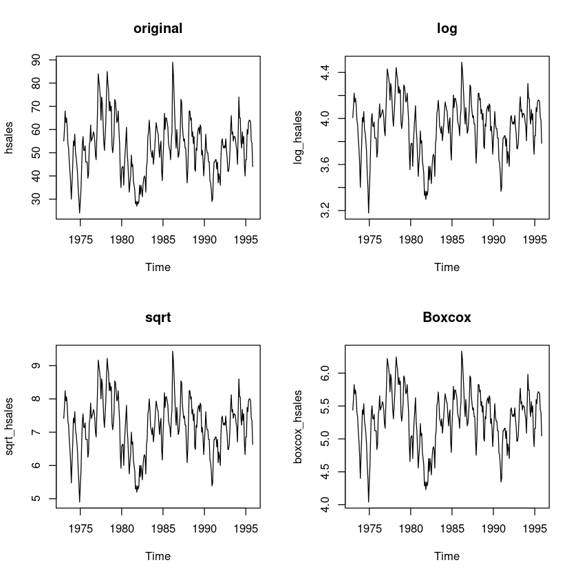

th = 1:length(hsales)
lmtest::bptest(lm(hsales~th)) #H0 : 등분산이다
lmtest::bptest(lm(log_hsales~th))
lmtest::bptest(lm(sqrt_hsales~th))
lmtest::bptest(lm(boxcox_hsales~th))

    studentized Breusch-Pagan test

data:  lm(hsales ~ th)
BP = 11.849, df = 1, p-value = 0.0005769

    studentized Breusch-Pagan test

data:  lm(log_hsales ~ th)
BP = 12.557, df = 1, p-value = 0.0003947

    studentized Breusch-Pagan test

data:  lm(sqrt_hsales ~ th)
BP = 12.834, df = 1, p-value = 0.0003403

    studentized Breusch-Pagan test

data:  lm(boxcox_hsales ~ th)
BP = 12.759, df = 1, p-value = 0.0003543

• 원데이터와 변환한데이터들간에 등분산은 큰 차이가 있어 보이진 않는다.

• 원데이터의 값의 범위가 크므로 log변환한 데이터를 사용한다.

forecast::tsdisplay(log_hsales)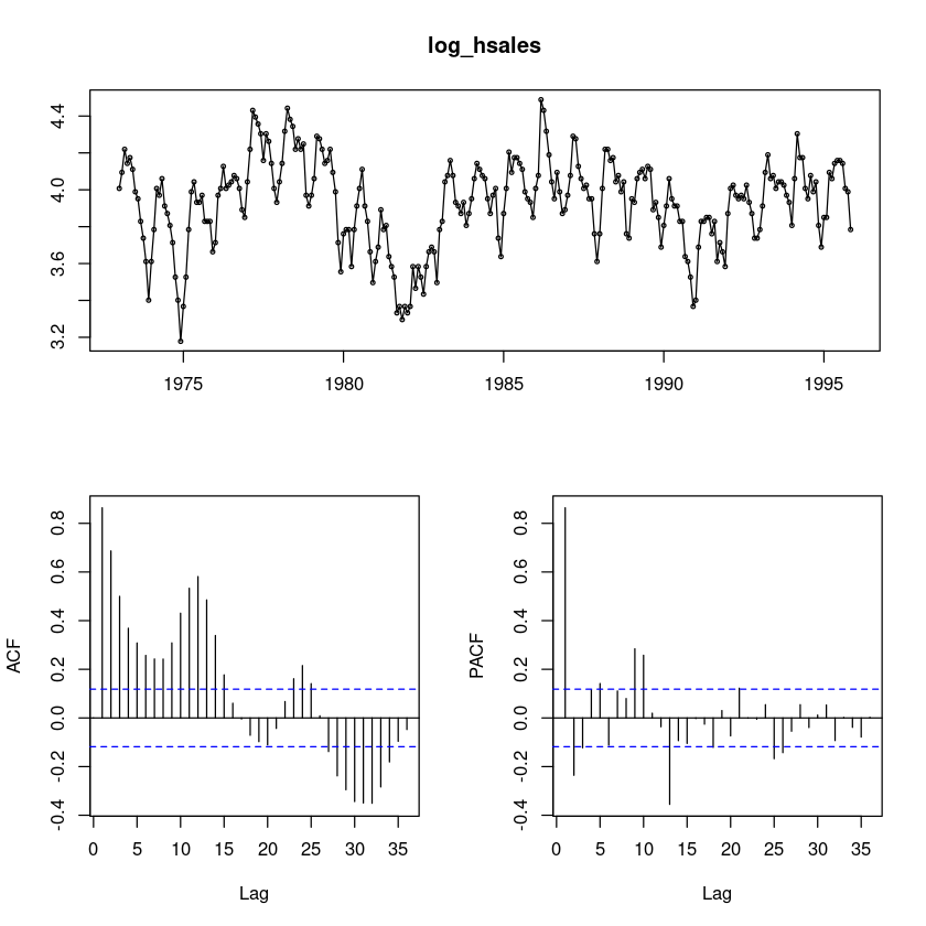

• SAR(2), AR(2)가 보이기도 하고..

• SMA(2)가 보이기도 한당

• 평균은 4 근처이다.

• ACF가 감소하고 있고 중간에 튀어나오는 부분들이 있어서 계절차분진행

• PACF가 유의한 부분이 몇개 보인다.

(3)

데이터가 정상시계열인가? 아니면 적절한 차분을 통해 정상시계열로 변환하여라

• 비정상시계열이다. 차분 진행

1

diff_log_hsales = diff(log_hsales)
forecast::tsdisplay(diff_log_hsales)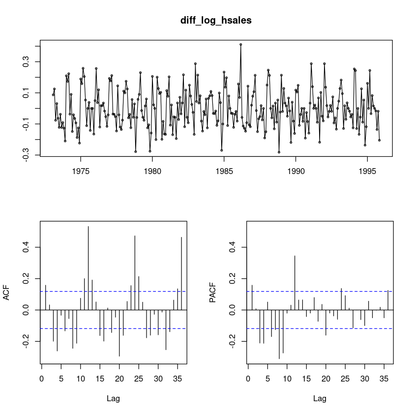

• 계절차분이 필요해 보인다.

diff1212_log_hsales = diff(diff(log_hsales),12)
forecast::tsdisplay(diff1212_log_hsales)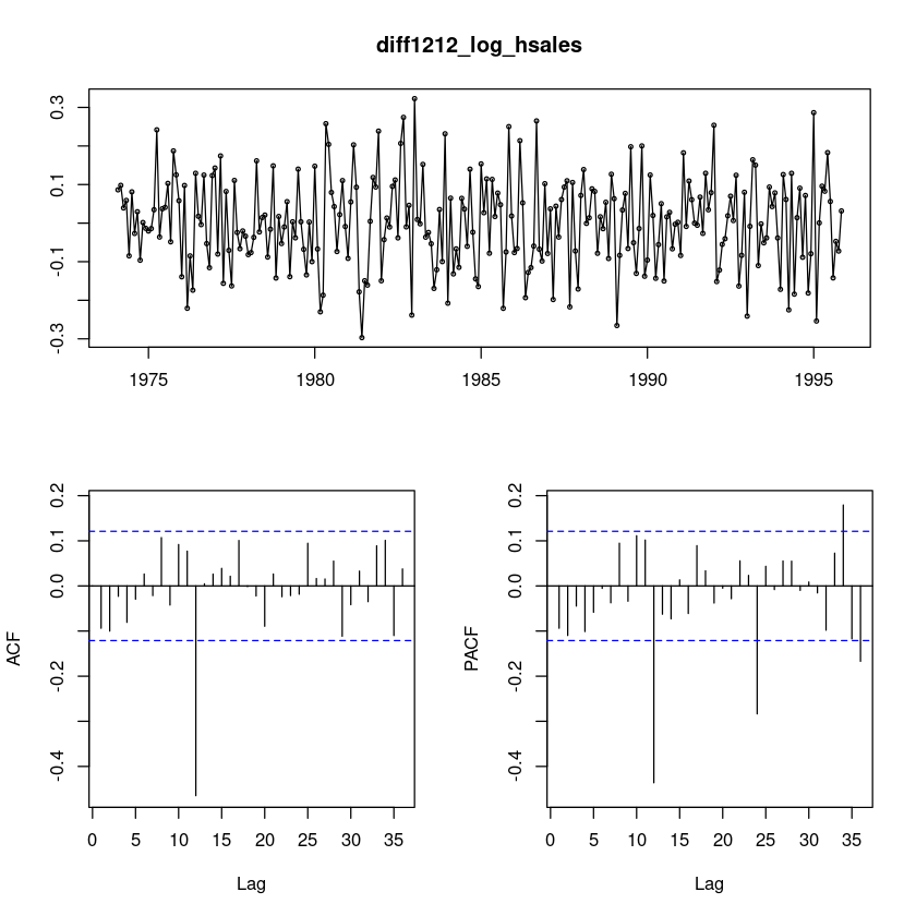

• diff1212_log_hsales: \(ARIMA(0,0,0)(0,0,1)_{12}\)이므로

• log_hsales: \(ARIMA(0,1,0)(0,1,1)_{12}\)

12

diff_log_hsales_12 = diff(log_hsales,12)
forecast::tsdisplay(diff_log_hsales_12)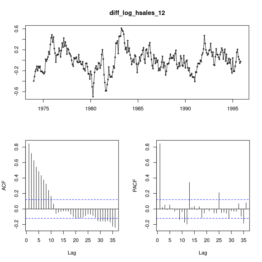

• ACF는 천천히 감소하는 형태이다. 계절차분을 했는데도 확률적 차분이 있어보인다. 한 번 더 차분을 해볼까?

• 평균은 0근처이다.

diff_log_hsales_12 = diff(diff(log_hsales,12))
forecast::tsdisplay(diff_log_hsales_12)

• 차분먼저 하고 -> 계쩔차분 한거랑.. 반대로 한거랑 비슷하게 나온당.

t.test(diff_log_hsales_12)

    One Sample t-test

data:  diff_log_hsales_12
t = 0.19616, df = 261, p-value = 0.8446
alternative hypothesis: true mean is not equal to 0
95 percent confidence interval:
 -0.01289978  0.01575430
sample estimates:
  mean of x 
0.001427261 

• 차분을 했더니 평균이 0이 되었다. t.test를 통해 0인것 확인

• 단위근 검정을 통해 차분이 더 필요한지 확인해 보기

##단위근 검정 : H0 : 단위근이 있다.
fUnitRoots::adfTest(diff_log_hsales_12, lags = 1, type = "nc")
fUnitRoots::adfTest(diff_log_hsales_12, lags = 2, type = "nc")

fUnitRoots::adfTest(diff_log_hsales_12, lags = 3, type = "nc")

Warning message in fUnitRoots::adfTest(diff_log_hsales_12, lags = 1, type = "nc"):
“p-value smaller than printed p-value”
Warning message in fUnitRoots::adfTest(diff_log_hsales_12, lags = 2, type = "nc"):
“p-value smaller than printed p-value”
Warning message in fUnitRoots::adfTest(diff_log_hsales_12, lags = 3, type = "nc"):
“p-value smaller than printed p-value”

Title:
 Augmented Dickey-Fuller Test

Test Results:
  PARAMETER:
    Lag Order: 1
  STATISTIC:
    Dickey-Fuller: -13.3169
  P VALUE:
    0.01 

Description:
 Tue Dec 12 21:26:53 2023 by user: 

Title:
 Augmented Dickey-Fuller Test

Test Results:
  PARAMETER:
    Lag Order: 2
  STATISTIC:
    Dickey-Fuller: -10.7125
  P VALUE:
    0.01 

Description:
 Tue Dec 12 21:26:53 2023 by user: 

Title:
 Augmented Dickey-Fuller Test

Test Results:
  PARAMETER:
    Lag Order: 3
  STATISTIC:
    Dickey-Fuller: -9.8584
  P VALUE:
    0.01 

Description:
 Tue Dec 12 21:26:53 2023 by user: 

유의확률이 작아서 차분을 할 필요가 없다!

정상시계열로 잘 변환된 것 같다.

(4)

모형을 식별하여라. (2개 이상의 모형 고려)(형태 : \(ARIMA(p.d.q)(P, D, Q)_s)\)

• diff1212_log_hsales: \(ARIMA(0,0,0)(0,0,1)_{12}\)이므로

• log_hsales: \(ARIMA(0,1,0)(0,1,1)_{12}\)

ARIMA(0,0,1)(1,0,0)_{12}도 생각

(5)

(4)에서 고려한 모형을 적합하여라.

fit6 = arima(log_hsales, order = c(0,1,0), include.mean=F,
     seasonal = list(order = c(0,1,1), period=12))
summary(fit6)
lmtest::coeftest(fit6)

Call:
arima(x = log_hsales, order = c(0, 1, 0), seasonal = list(order = c(0, 1, 1), 
    period = 12), include.mean = F)

Coefficients:
         sma1
      -0.9999
s.e.   0.0801

sigma^2 estimated as 0.007124:  log likelihood = 257.18,  aic = -510.35

Training set error measures:
                      ME       RMSE        MAE        MPE     MAPE    MASE
Training set 0.003952528 0.08239128 0.06409028 0.08562818 1.645261 0.64136
                   ACF1
Training set -0.1038561

z test of coefficients:

      Estimate Std. Error z value  Pr(>|z|)    
sma1 -0.999931   0.080144 -12.477 < 2.2e-16 ***
---
Signif. codes:  0 ‘***’ 0.001 ‘**’ 0.01 ‘*’ 0.05 ‘.’ 0.1 ‘ ’ 1

fit3 = arima(log_hsales, order = c(0,1,1), include.mean=F,
     seasonal = list(order = c(0,1,1), period=12))
summary(fit3)
lmtest::coeftest(fit3)

Call:
arima(x = log_hsales, order = c(0, 1, 1), seasonal = list(order = c(0, 1, 1), 
    period = 12), include.mean = F)

Coefficients:
          ma1     sma1
      -0.1111  -1.0000
s.e.   0.0656   0.0765

sigma^2 estimated as 0.007046:  log likelihood = 258.6,  aic = -511.21

Training set error measures:
                      ME       RMSE        MAE        MPE     MAPE      MASE
Training set 0.004407847 0.08194001 0.06413126 0.09625902 1.647035 0.6417701
                      ACF1
Training set -0.0006868962

z test of coefficients:

      Estimate Std. Error z value Pr(>|z|)    
ma1  -0.111134   0.065604  -1.694  0.09026 .  
sma1 -0.999971   0.076478 -13.075  < 2e-16 ***
---
Signif. codes:  0 ‘***’ 0.001 ‘**’ 0.01 ‘*’ 0.05 ‘.’ 0.1 ‘ ’ 1

fit4 <- forecast::auto.arima(ts(log_hsales, frequency=12),
                     test = "adf",
                     seasonal = TRUE, trace = F)
summary(fit4)
lmtest::coeftest(fit4)

Series: ts(log_hsales, frequency = 12) 
ARIMA(2,0,2)(2,1,0)[12] with drift 

Coefficients:
         ar1     ar2     ma1      ma2     sar1     sar2    drift
      0.0498  0.8203  0.8434  -0.0280  -0.6244  -0.3207  -0.0005
s.e.  0.3203  0.2978  0.3281   0.0737   0.0617   0.0615   0.0035

sigma^2 = 0.009325:  log likelihood = 241.64
AIC=-467.28   AICc=-466.71   BIC=-438.7

Training set error measures:
                      ME       RMSE        MAE         MPE     MAPE      MASE
Training set 0.001548434 0.09317171 0.07411262 0.005293838 1.907259 0.4415353
                     ACF1
Training set -0.008857548

z test of coefficients:

        Estimate Std. Error  z value  Pr(>|z|)    
ar1    0.0497676  0.3203457   0.1554  0.876541    
ar2    0.8202974  0.2978056   2.7545  0.005879 ** 
ma1    0.8433986  0.3281198   2.5704  0.010158 *  
ma2   -0.0280483  0.0737334  -0.3804  0.703647    
sar1  -0.6243889  0.0617155 -10.1172 < 2.2e-16 ***
sar2  -0.3206978  0.0614554  -5.2184 1.805e-07 ***
drift -0.0004683  0.0034659  -0.1351  0.892520    
---
Signif. codes:  0 ‘***’ 0.001 ‘**’ 0.01 ‘*’ 0.05 ‘.’ 0.1 ‘ ’ 1

(6)

(5)에서 적합된 결과를 이용하여 더 좋은 모형을 선택하여라

• \(ARIMA(0,1,1)(0,1,1)_{12}\)

(7)

(6)에서 선택한 모형을 이용하여 잔차검정을 시행하여라

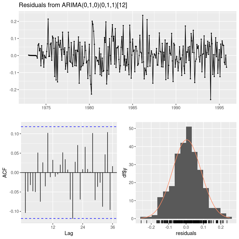
forecast::checkresiduals(fit6)

    Ljung-Box test

data:  Residuals from ARIMA(0,1,0)(0,1,1)[12]
Q* = 21.749, df = 23, p-value = 0.5355

Model df: 1.   Total lags used: 24

t.test(resid(fit6))

    One Sample t-test

data:  resid(fit6)
t = 0.795, df = 274, p-value = 0.4273
alternative hypothesis: true mean is not equal to 0
95 percent confidence interval:
 -0.005835073  0.013740130
sample estimates:
  mean of x 
0.003952528 

잔차 평균 0

#모형 적합도 검정 : H0 : rho1=...=rho_k=0
Box.test(resid(fit6), lag=1, type = "Ljung-Box")
Box.test(resid(fit6), lag=6, type = "Ljung-Box")
Box.test(resid(fit6), lag=12, type = "Ljung-Box")

    Box-Ljung test

data:  resid(fit6)
X-squared = 2.9987, df = 1, p-value = 0.08333

    Box-Ljung test

data:  resid(fit6)
X-squared = 6.0675, df = 6, p-value = 0.4157

    Box-Ljung test

data:  resid(fit6)
X-squared = 11.569, df = 12, p-value = 0.4809

fit6

Call:
arima(x = log_hsales, order = c(0, 1, 0), seasonal = list(order = c(0, 1, 1), 
    period = 12), include.mean = F)

Coefficients:
         sma1
      -0.9999
s.e.   0.0801

sigma^2 estimated as 0.007124:  log likelihood = 257.18,  aic = -510.35

aic가 큰 차이가 없어서.. 그냥 모형 간단한 fit6

lmtest::coeftest(fit6) 

z test of coefficients:

      Estimate Std. Error z value  Pr(>|z|)    
sma1 -0.999931   0.080144 -12.477 < 2.2e-16 ***
---
Signif. codes:  0 ‘***’ 0.001 ‘**’ 0.01 ‘*’ 0.05 ‘.’ 0.1 ‘ ’ 1

(8)

다음 2년간의 주택의 월별 거래량을 예측하여라.

fore_fit <- forecast::forecast(fit6, 24)

fore_fit

         Point Forecast    Lo 80    Hi 80    Lo 95    Hi 95
Dec 1995       3.692314 3.581718 3.802911 3.523171 3.861457
Jan 1996       3.820471 3.664063 3.976878 3.581266 4.059675
Feb 1996       3.941495 3.749996 4.132993 3.648622 4.234367
Mar 1996       4.120349 3.899260 4.341438 3.782223 4.458475
Apr 1996       4.097816 3.850655 4.344978 3.719815 4.475817
May 1996       4.096899 3.826164 4.367634 3.682846 4.510952
Jun 1996       4.052821 3.760407 4.345234 3.605612 4.500029
Jul 1996       3.995515 3.682922 4.308108 3.517445 4.473584
Aug 1996       4.018546 3.687000 4.350092 3.511490 4.525602
Sep 1996       3.934200 3.584727 4.283673 3.399727 4.468673
Oct 1996       3.913847 3.547323 4.280371 3.353297 4.474397
Nov 1996       3.776082 3.393265 4.158898 3.190614 4.361549
Dec 1996       3.684206 3.284402 4.084011 3.072758 4.295654
Jan 1997       3.812363 3.396263 4.228462 3.175993 4.448732
Feb 1997       3.933387 3.501687 4.365086 3.273159 4.593614
Mar 1997       4.112241 3.665485 4.558996 3.428987 4.795495
Apr 1997       4.089708 3.628388 4.551029 3.384180 4.795237
May 1997       4.088791 3.613352 4.564230 3.361670 4.815913
Jun 1997       4.044712 3.555562 4.533863 3.296621 4.792804
Jul 1997       3.987407 3.484919 4.489895 3.218917 4.755896
Aug 1997       4.010438 3.494958 4.525919 3.222079 4.798798
Sep 1997       3.926092 3.397939 4.454245 3.118351 4.733833
Oct 1997       3.905739 3.365209 4.446268 3.079071 4.732407
Nov 1997       3.767974 3.215346 4.320602 2.922802 4.613145

exp(fore_fit$mean)

A Time Series: 3 × 12

	Jan	Feb	Mar	Apr	May	Jun	Jul	Aug	Sep	Oct	Nov	Dec
1995												40.13763
1996	45.62569	51.49551	61.58072	60.20867	60.15348	57.55958	54.35380	55.62019	51.12123	50.09127	43.64469	39.81351
1997	45.25725	51.07967	61.08344	59.72247	59.66772	57.09477	53.91488	55.17104	50.70842	49.68677	43.29224

- 그림은 그냥 log변환했던 그림으로..

plot(fore_fit)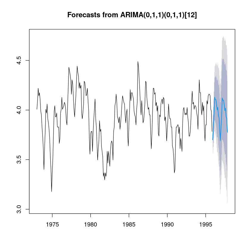

6

(R실습) 영국의 분기별 승용차 생산 대수 (단위 : 천 대) 자료(expsmooth::ukcars)에 대하여 다음 물음에 답하여라.

install.packages("expsmooth")
library(expsmooth)

Installing package into ‘/home/coco/R/x86_64-pc-linux-gnu-library/4.2’
(as ‘lib’ is unspecified)

(1)

시계열 그림을 그리시오.

forecast::tsdisplay(ukcars,lag.max=40)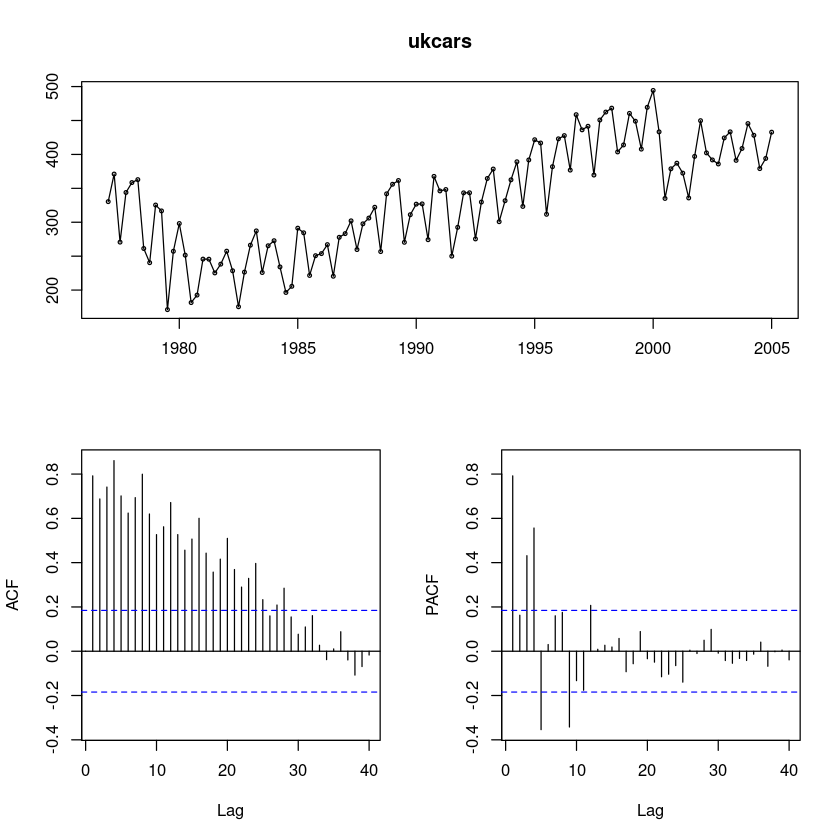

• acf가 중간중에 튀어나오는게 보인다. 계절차분.. 주기가 4인것 같다.

(2)

변수변환이 필요한지를 설명하고, 필요하다면 적절한 변수 변환을 하여라.

log_ukcars = log(ukcars)
sqrt_ukcars = sqrt(ukcars)
boxcox_ukcars = forecast::BoxCox(ukcars,lambda= forecast::BoxCox.lambda(ukcars))

par(mfrow=c(2,2))
plot.ts(ukcars, main = "original")
plot.ts(log_ukcars, main = 'log')
plot.ts(sqrt_ukcars, main = 'sqrt')
plot.ts(boxcox_ukcars, main = 'Boxcox')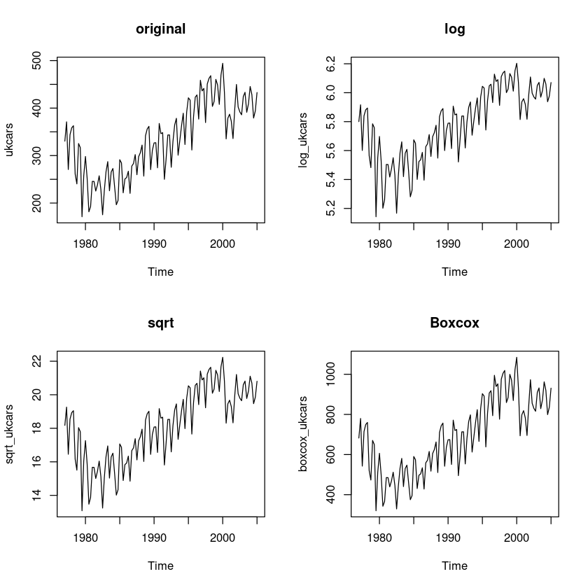

t = 1:length(ukcars)
lmtest::bptest(lm(ukcars~t)) #H0 : 등분산이다
lmtest::bptest(lm(log_ukcars~t))
lmtest::bptest(lm(sqrt_ukcars~t))
lmtest::bptest(lm(boxcox_ukcars~t))

    studentized Breusch-Pagan test

data:  lm(ukcars ~ t)
BP = 9.389, df = 1, p-value = 0.002183

    studentized Breusch-Pagan test

data:  lm(log_ukcars ~ t)
BP = 20.839, df = 1, p-value = 4.997e-06

    studentized Breusch-Pagan test

data:  lm(sqrt_ukcars ~ t)
BP = 15.696, df = 1, p-value = 7.439e-05

    studentized Breusch-Pagan test

data:  lm(boxcox_ukcars ~ t)
BP = 7.5728, df = 1, p-value = 0.005926

ARIMA(1,0,1)(2,0,0)_4 아닐지도..

##단위근 검정 : H0 : 단위근이 있다.
fUnitRoots::adfTest(diff4_log_ukcars, lags = 0, type = "nc")
fUnitRoots::adfTest(diff4_log_ukcars, lags = 1, type = "nc")
fUnitRoots::adfTest(diff4_log_ukcars, lags = 2, type = "nc")

Warning message in fUnitRoots::adfTest(diff4_log_ukcars, lags = 0, type = "nc"):
“p-value smaller than printed p-value”
Warning message in fUnitRoots::adfTest(diff4_log_ukcars, lags = 1, type = "nc"):
“p-value smaller than printed p-value”
Warning message in fUnitRoots::adfTest(diff4_log_ukcars, lags = 2, type = "nc"):
“p-value smaller than printed p-value”

Title:
 Augmented Dickey-Fuller Test

Test Results:
  PARAMETER:
    Lag Order: 0
  STATISTIC:
    Dickey-Fuller: -6.2158
  P VALUE:
    0.01 

Description:
 Wed Dec 13 14:05:45 2023 by user: 

Title:
 Augmented Dickey-Fuller Test

Test Results:
  PARAMETER:
    Lag Order: 1
  STATISTIC:
    Dickey-Fuller: -5.6776
  P VALUE:
    0.01 

Description:
 Wed Dec 13 14:05:45 2023 by user: 

Title:
 Augmented Dickey-Fuller Test

Test Results:
  PARAMETER:
    Lag Order: 2
  STATISTIC:
    Dickey-Fuller: -5.9791
  P VALUE:
    0.01 

Description:
 Wed Dec 13 14:05:45 2023 by user: 

• pvalue값이 0.05보다 작으므로 차분이 필요하지 않다

t.test(diff4_log_ukcars)

    One Sample t-test

data:  diff4_log_ukcars
t = 0.65613, df = 108, p-value = 0.5131
alternative hypothesis: true mean is not equal to 0
95 percent confidence interval:
 -0.01643180  0.03269295
sample estimates:
  mean of x 
0.008130578 

• 평균이 0이다.

(3)

마지막 2년동안의 데이터는 test데이터, 나머지는 train 데이터로 분할하여라

uk_tr <- head(log_ukcars,-8)
uk_ts <- tail(log_ukcars,8)

uk_tr # train

A Time Series: 27 × 4

	Qtr1	Qtr2	Qtr3	Qtr4
1977	5.800216	5.916340	5.600900	5.840293
1978	5.881904	5.893912	5.565596	5.482117
1979	5.785000	5.757955	5.142558	5.549920
1980	5.697520	5.527300	5.201559	5.260605
1981	5.503916	5.503403	5.417260	5.473157
1982	5.550573	5.431366	5.166904	5.422577
1983	5.584060	5.660356	5.420017	5.580910
1984	5.608589	5.455894	5.280469	5.325694
1985	5.674295	5.650459	5.400743	5.524245
1986	5.536377	5.587309	5.395390	5.626905
1987	5.646270	5.710665	5.559604	5.695945
1988	5.724007	5.774881	5.547998	5.834451
1989	5.874942	5.890373	5.600024	5.740130
1990	5.789006	5.790141	5.614066	5.907012
1991	5.846910	5.852809	5.521493	5.678526
1992	5.838657	5.838980	5.618174	5.798326
1993	5.898584	5.936079	5.706439	5.804403
1994	5.893124	5.963921	5.778649	5.970833
1995	6.044166	6.032662	5.742083	5.945164
1996	6.047330	6.058473	5.931847	6.128135
1997	6.078158	6.090149	5.912329	6.110853
1998	6.136521	6.148964	6.000513	6.025740
1999	6.132304	6.106871	6.010745	6.151472
2000	6.203165	6.071292	5.814447	5.936995
2001	5.958683	5.919955	5.816486	5.984138
2002	6.108703	5.997079	5.970871	5.955552
2003	6.050500

uk_ts # test

A Time Series: 3 × 4

	Qtr1	Qtr2	Qtr3	Qtr4
2003		6.071384	5.969252	6.013079
2004	6.099103	6.059595	5.937663	5.976458
2005	6.070266

(4)

train 데이터에 이동평균 모형을 적합하고, 마지막 2년의 승용차 생산 대수를 예측하여라.

fitt <- SMA(uk_tr,10)

forecast(tail(fitt,-9),8)

        Point Forecast    Lo 80    Hi 80    Lo 95    Hi 95
2003 Q2       5.976598 5.958328 5.994868 5.948657 6.004539
2003 Q3       5.966925 5.930276 6.003575 5.910874 6.022977
2003 Q4       5.965189 5.905953 6.024426 5.874595 6.055784
2004 Q1       5.987854 5.903003 6.072705 5.858086 6.117622
2004 Q2       5.993410 5.879633 6.107187 5.819403 6.167416
2004 Q3       5.982569 5.840527 6.124611 5.765334 6.199803
2004 Q4       5.979765 5.808140 6.151391 5.717287 6.242244
2005 Q1       6.001492 5.798600 6.204384 5.691195 6.311789

fitt_<-forecast(tail(fitt,-9),8)
fit1_mean<-exp(fitt_$mean)
fit1_mean

A Time Series: 3 × 4

	Qtr1	Qtr2	Qtr3	Qtr4
2003		394.0974	390.3038	389.6268
2004	398.5584	400.7789	396.4574	395.3476
2005	404.0312

plot(forecast(tail(fitt,-9),8))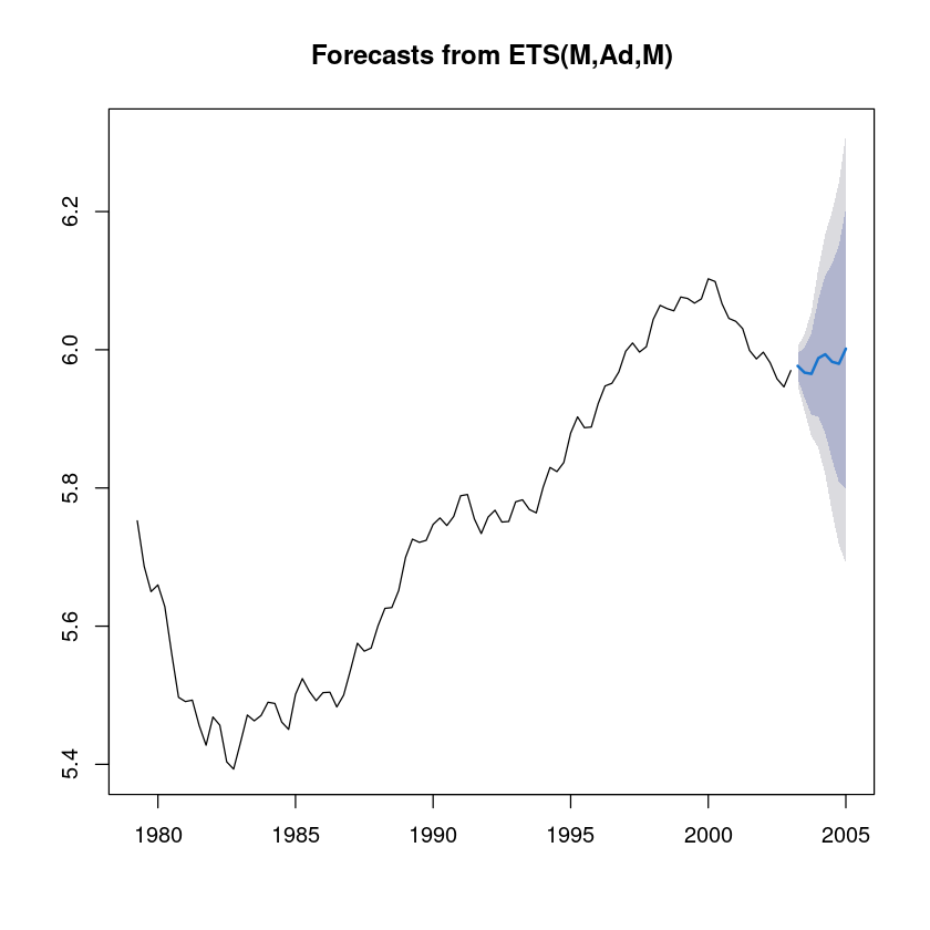

(5)

train 데이터에 지수평활 모형을 적합하고, 마지막 2년의 승용차 생산 대수예측하여라

fit2=HoltWinters(uk_tr) 
fit2

Holt-Winters exponential smoothing with trend and additive seasonal component.

Call:
HoltWinters(x = uk_tr)

Smoothing parameters:
 alpha: 0.5359051
 beta : 0.03931353
 gamma: 0.280097

Coefficients:
           [,1]
a   5.958690456
b   0.001696387
s1  0.069343432
s2 -0.085652720
s3  0.025071836
s4  0.096844294

fit2_2=forecast(fit2, h=8)
plot(fit2_2)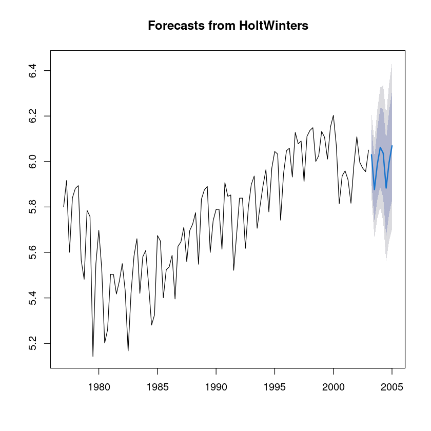

fit2_2

        Point Forecast    Lo 80    Hi 80    Lo 95    Hi 95
2003 Q2       6.029730 5.907757 6.151703 5.843189 6.216272
2003 Q3       5.876431 5.736814 6.016047 5.662906 6.089955
2003 Q4       5.988851 5.832443 6.145260 5.749645 6.228058
2004 Q1       6.062320 5.889683 6.234958 5.798294 6.326346
2004 Q2       6.036516 5.841129 6.231902 5.737698 6.335334
2004 Q3       5.883216 5.672756 6.093676 5.561345 6.205087
2004 Q4       5.995637 5.770205 6.221069 5.650868 6.340406
2005 Q1       6.069106 5.828757 6.309455 5.701524 6.436688

fit2_mean <- exp(fit2_2$mean)
fit2_mean

A Time Series: 3 × 4

	Qtr1	Qtr2	Qtr3	Qtr4
2003		415.6029	356.5343	398.9561
2004	429.3706	418.4326	358.9618	401.6725
2005	432.2940

(6)

train 데이터에 계절형 ARIMA 모형을 적합하고, 마지막 2년의 승용차 생산 대수 예측하여라.

fit3 <- forecast::auto.arima(ts(uk_tr, frequency=4),
                     test = "adf",
                     seasonal = TRUE, trace = T)
fit3

 ARIMA(2,0,2)(1,1,1)[4] with drift         : Inf
 ARIMA(0,0,0)(0,1,0)[4] with drift         : -116.3653
 ARIMA(1,0,0)(1,1,0)[4] with drift         : -172.5345
 ARIMA(0,0,1)(0,1,1)[4] with drift         : -157.3235
 ARIMA(0,0,0)(0,1,0)[4]                    : -118.0766
 ARIMA(1,0,0)(0,1,0)[4] with drift         : -139.6757
 ARIMA(1,0,0)(2,1,0)[4] with drift         : -176.0384
 ARIMA(1,0,0)(2,1,1)[4] with drift         : -177.9085
 ARIMA(1,0,0)(1,1,1)[4] with drift         : -180.1665
 ARIMA(1,0,0)(0,1,1)[4] with drift         : -179.5978
 ARIMA(1,0,0)(1,1,2)[4] with drift         : -178.205
 ARIMA(1,0,0)(0,1,2)[4] with drift         : -180.1353
 ARIMA(1,0,0)(2,1,2)[4] with drift         : -176.0221
 ARIMA(0,0,0)(1,1,1)[4] with drift         : -132.7479
 ARIMA(2,0,0)(1,1,1)[4] with drift         : -181.6961
 ARIMA(2,0,0)(0,1,1)[4] with drift         : -180.0464
 ARIMA(2,0,0)(1,1,0)[4] with drift         : -172.5136
 ARIMA(2,0,0)(2,1,1)[4] with drift         : -179.6537
 ARIMA(2,0,0)(1,1,2)[4] with drift         : -180.4408
 ARIMA(2,0,0)(0,1,0)[4] with drift         : -138.1924
 ARIMA(2,0,0)(0,1,2)[4] with drift         : -181.1778
 ARIMA(2,0,0)(2,1,0)[4] with drift         : -175.4253
 ARIMA(2,0,0)(2,1,2)[4] with drift         : -178.0885
 ARIMA(3,0,0)(1,1,1)[4] with drift         : -180.5785
 ARIMA(2,0,1)(1,1,1)[4] with drift         : -181.1476
 ARIMA(1,0,1)(1,1,1)[4] with drift         : -183.0138
 ARIMA(1,0,1)(0,1,1)[4] with drift         : -180.5136
 ARIMA(1,0,1)(1,1,0)[4] with drift         : -173.0476
 ARIMA(1,0,1)(2,1,1)[4] with drift         : -181.3413
 ARIMA(1,0,1)(1,1,2)[4] with drift         : -182.1301
 ARIMA(1,0,1)(0,1,0)[4] with drift         : -137.9048
 ARIMA(1,0,1)(0,1,2)[4] with drift         : -182.1227
 ARIMA(1,0,1)(2,1,0)[4] with drift         : -175.9096
 ARIMA(1,0,1)(2,1,2)[4] with drift         : -179.7711
 ARIMA(0,0,1)(1,1,1)[4] with drift         : -157.0855
 ARIMA(1,0,2)(1,1,1)[4] with drift         : -181.1722
 ARIMA(0,0,2)(1,1,1)[4] with drift         : -161.9388
 ARIMA(1,0,1)(1,1,1)[4]                    : -185.1282
 ARIMA(1,0,1)(0,1,1)[4]                    : -181.64
 ARIMA(1,0,1)(1,1,0)[4]                    : -175.0856
 ARIMA(1,0,1)(2,1,1)[4]                    : -183.3356
 ARIMA(1,0,1)(1,1,2)[4]                    : -184.1763
 ARIMA(1,0,1)(0,1,0)[4]                    : -139.9217
 ARIMA(1,0,1)(0,1,2)[4]                    : -184.2699
 ARIMA(1,0,1)(2,1,0)[4]                    : -178.0297
 ARIMA(1,0,1)(2,1,2)[4]                    : -181.8691
 ARIMA(0,0,1)(1,1,1)[4]                    : -158.4394
 ARIMA(1,0,0)(1,1,1)[4]                    : -181.3926
 ARIMA(2,0,1)(1,1,1)[4]                    : -183.3919
 ARIMA(1,0,2)(1,1,1)[4]                    : -183.4158
 ARIMA(0,0,0)(1,1,1)[4]                    : -134.1378
 ARIMA(0,0,2)(1,1,1)[4]                    : -163.1242
 ARIMA(2,0,0)(1,1,1)[4]                    : -183.4676
 ARIMA(2,0,2)(1,1,1)[4]                    : -181.1076

 Best model: ARIMA(1,0,1)(1,1,1)[4]                    

Series: ts(uk_tr, frequency = 4) 
ARIMA(1,0,1)(1,1,1)[4] 

Coefficients:
         ar1      ma1     sar1     sma1
      0.9323  -0.3616  -0.3205  -0.6647
s.e.  0.0521   0.1286   0.1273   0.1251

sigma^2 = 0.008448:  log likelihood = 97.88
AIC=-185.76   AICc=-185.13   BIC=-172.68

fore_fit <- forecast::forecast(fit3, 8)
plot(fore_fit)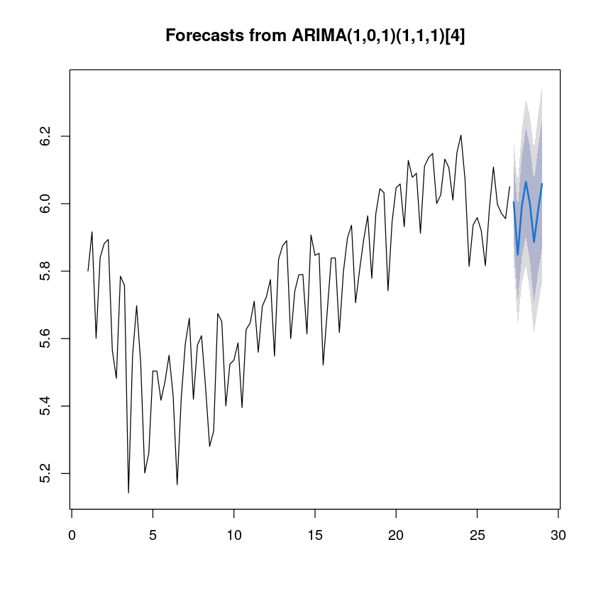

fit3_mean <- exp(fore_fit$mean)
fit3_mean

A Time Series: 3 × 4

	Qtr1	Qtr2	Qtr3	Qtr4
27		405.2362	346.7585	399.9905
28	430.3242	403.6273	360.0729	394.8634
29	427.8340

(7)

(3)-(5) 모형의 결과에 대하여 MSE/MAPE/MAE를 구하고, 가장 좋은 모형을 선택하여라

test<-exp(uk_ts)

mse1 <- mean((fit1_mean - test)^2)
mse2 <- mean((fit2_mean - test)^2)
mse3 <- mean((as.numeric(fit3_mean) - as.numeric(test))^2)
mse1
mse2
mse3

748.153071542761

303.373955852896

507.188544601796

mape1 <- mean(abs((fit1_mean - test)/test))*100
mape2 <- mean(abs((fit2_mean - test)/test))*100
mape3 <- mean(abs((as.numeric(fit3_mean) - as.numeric(test))/as.numeric(test)))*100
mape1
mape2
mape3

5.30687182638847

3.57279927836919

4.43420488223284

mae1 <- mean(abs(test-fit1_mean))
mae2 <- mean(abs(test-fit2_mean))
mae3 <- mean(abs(as.numeric(test)-as.numeric(fit3_mean)))
mae1
mae2
mae3

22.6259439951361

14.5268936719517

18.2143508191435